Tutorial 2: Modal Analysis

Goals of the tutorial

In this tutorial, we will do an eigenvalue decomposition of the base flow obtained in the tutorial of cylinder wake. By the end of this tutorial, you will be able to:

• Define the boundary conditions.

• Run a linear stability analysis case.

• Postprocess modal analysis results with paraview.

The linear stability analysis provides insights into:

• The growth or decay rates of small perturbations superimposed on the base flow.

• The dominant spatial structures (modes) associated with flow instabilities.

The modal analysis will:

1. Identify which flow structures are most likely to become unstable.

2. Quantify the stability characteristics by computing eigenvalues and corresponding eigenmodes.

Requirements

Before you begin this tutorial make sure to:

• have completed the base flow tutorial.

• access the case folder felics/tutorials/modal_analysis_tutorial and copy it into your working directory.

Modal analysis settings

Boundary conditions

The boundary conditions for the fluctuations are:

Boundary	ID	\(u'_x\)	\(u'_y\)	\(p'\)
Inlet	1	Dirichlet	Dirichlet	Dirichlet
Symmetry	2	Dirichlet	Neumann	Dirichlet
Outlet	3	Dirichlet	Dirichlet	Dirichlet
Top	4	Dirichlet	Dirichlet	Dirichlet
Wall	5	Dirichlet	Dirichlet	Neumann

Note

The BCs for the base flow variables (\(\bar{u}_x, \bar{u}_y, \bar{p}\)) in base flow tutorial and for the perturbations (\(u_x', u_y', p'\)) current modal analysis are different. ‘’’

These BCs are implemented in bc_modal.json using different names.

When all BCs are set to Dirichlet with a value 0 (always the case for fluctuations), we set:

    "1": {
        "name": "zeroDirichlet"
    },

We impose this for Inlet, Outlet, Top. To impose a symmetric boundary condition we specify the BC for every variable:

    "2":{
        "name": "symmetry",
        "specifics": [
        {
            "type": "Dirichlet",
            "value": 0.0,
            "variable": "ux"
        },
        {
            "type": "Neumann",
            "value": 0.0,
            "variable": "uy"
        },
        {
            "type": "Dirichlet",
            "value": 0.0,
            "variable": "p"
        }
        ]
    },

The wall BC is imposed with:

    "5":{
        "name": "wall"
    }

The complete structure of this file is detailed in Setting files.

Settings

The setting file, modal.json contains all the information relevant for modal analysis. The detailed structure of modal.json can be found inside FELiCS settings.

Here are some key settings for our resolvent analysis:

• The spanwise wavenumber is set to 0:

{"m": 0.0,}

• We specify the spatial domain dimension in the settings file as 2D:

{"nDim": 2}

• The coordinate system is set to Cartesian:

{"CoordinateSystem": "Cartesian"}

• We include the mesh file cylinder_wake.msh, the base flow file base_flow_for_FELiCS.fel generated in the base flow tutorial and the BCs file bc_modal.json with these references:

{"MeshFilePath":"cylinder_wake.msh"}
{"MeanFlowFilePath": "base_flow_for_FELiCS.fel"}
{"BCsFilePath": "bc_modal.json"}

• We specify which eigenvalues to compute by providing a list of initial guesses:

{"EigenValueGuess": [0.7]}

• For each guess, the number of eigenvalues to be calculated closest to that value is set to:

{"nSolut": 100}

Running the analysis

Run the modal analysis via

FELiCS -f modal.json

Postprocessing

After running the modal analysis, the working directory should look like:

.
└── logs
└── output_dir
├ base_flow_for_FELiCS.fel
├ bc_modal.json
├ cylinder_wake.msh
├ modal.json
├ PlotScatter.py
└ ...

Inside the output_dir directory, all the eigenmodes in .h5 and .xmf format can be found, along with the eigenvalues in spectrum.csv file. Run the pyhton script PlotScatter.py to plot the computed eigenvalue spectrum: 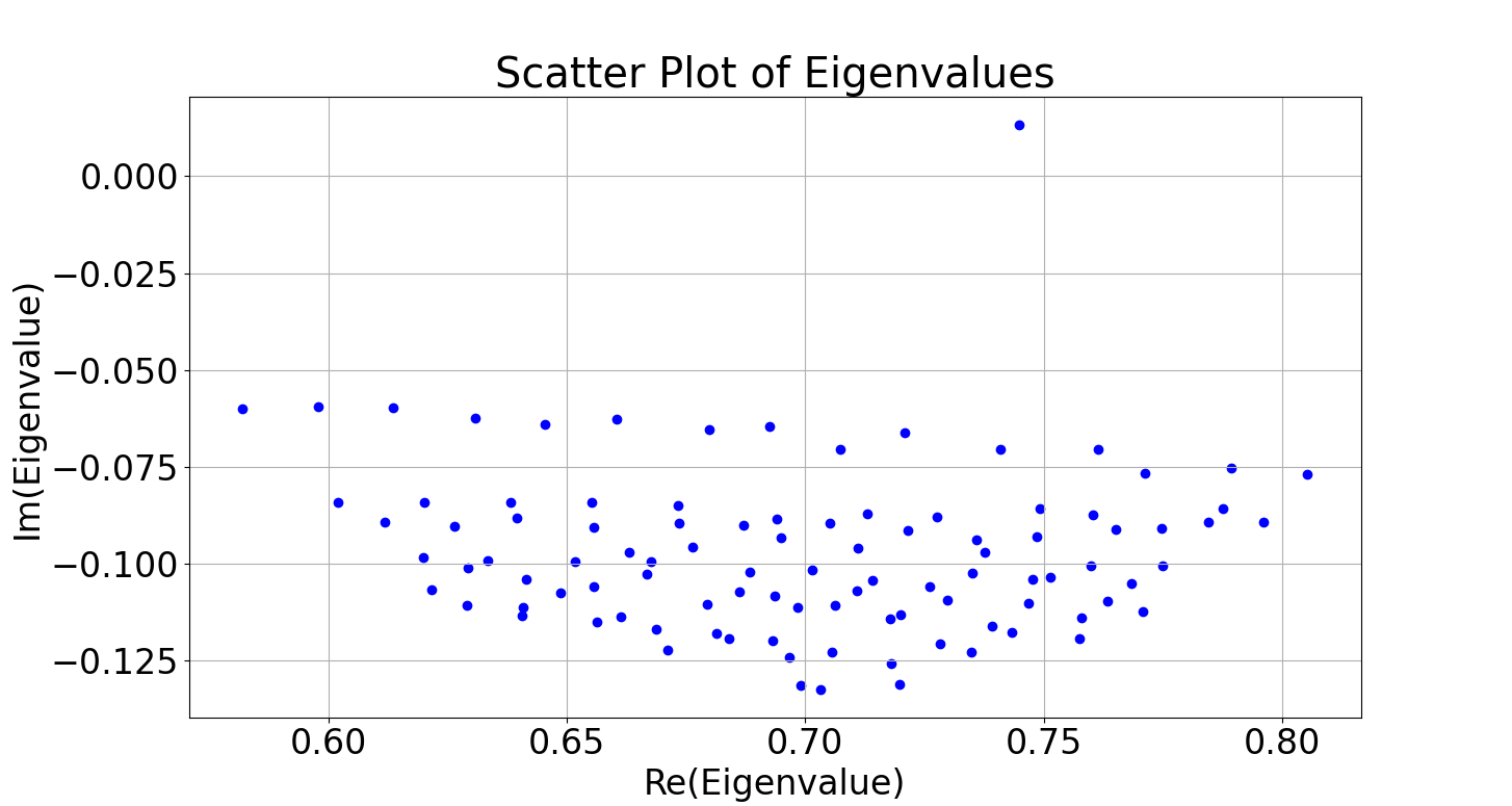Figure 1. Eigenspectrum

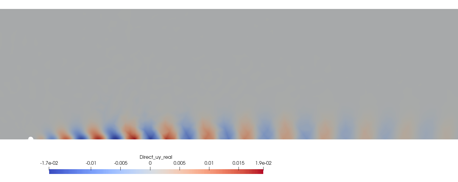
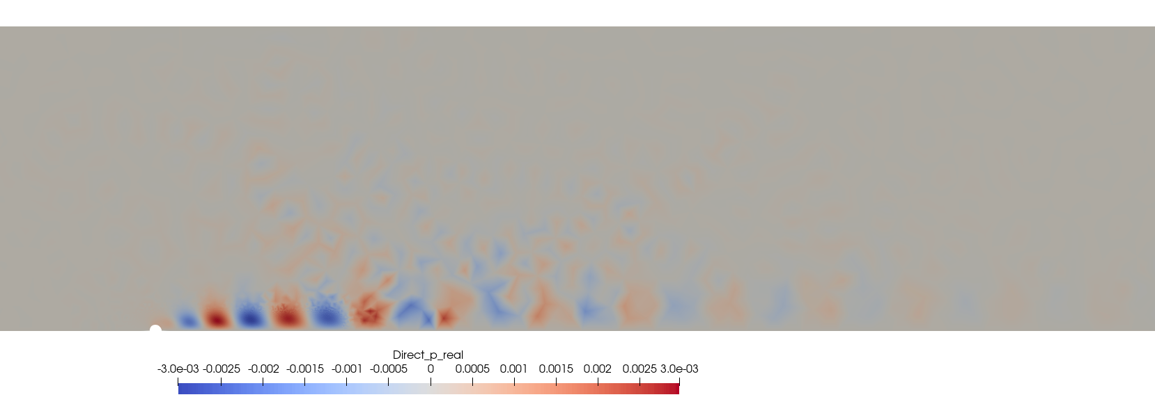
In Figure 1, an eigenvalue with a positive imaginary part stands out. We use paraview to visualize the corresponding real part of the eigenmode stored in Mode_Modal_Direct_Omega_0.745+0.013j.xmf.

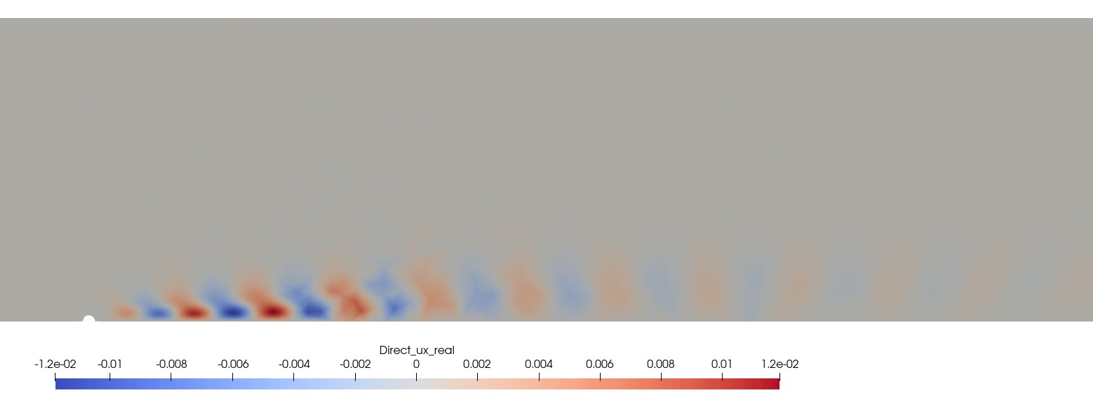Figure 2. Real eigenmode, \(u'_x\)

Figure 3. Real eigenmode, \(u'_y\)

Figure 4. Real eigenmode, \(p'\)