Tutorial 1: Solve the base flow

Goals of the tutorial

This first tutorial gives an introduction for setting up a FELiCS case. By the end of this tutorial, you will be able to:

• Define a case in FELiCS.

• Create a case folder with a mesh and base flow files.

Requirements

• FELiCS should be installed as per the FELiCS installation guide with an active conda environment.

• Choose a branch of the FELiCS that contains the base flow solver.

Case Definition

We want to study the linear stability of a 2D base flow around a cylinder at Reynolds number, \(\mathrm{Re} = 50\). In general it is recommended to create a folder for every case, where the input and output files will be located. Here, the case folder can be found in felics/tutorials/cylinder_wake_tutorial. Copy this tutorial to your working directory workDir

cp -r felics/tutorials/cylinder_wake_tutorial workDir/
cd workDir/cylinder_wake_tutorial/ 

Mesh generation

Since the code uses the Finite Element Continuous Galerkin approach, a computational grid needs to be created. In order to create the mesh, the package python-gmsh is used. An input file for this program called cylinder_wake_mesh.py is already prepared in the folder. Upon exceuting it in python it generates the mesh file cylinder_wake.msh in Version 2 ASCII format.

python cylinder_wake_mesh.py

If you open the mesh in GMSH, click on Mesh -> 2D. It should look like:

Figure 1. 2D Mesh.

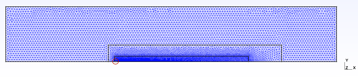
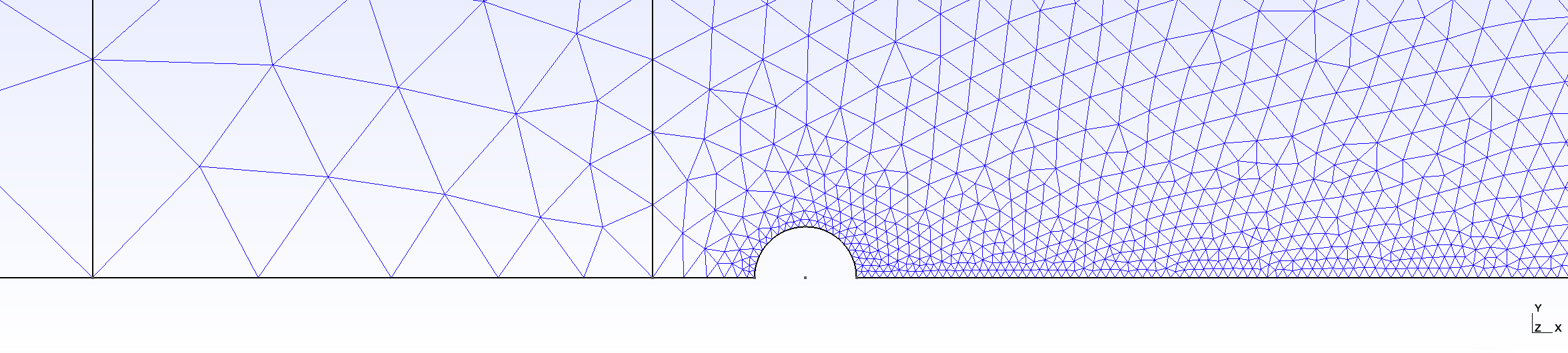Figure 2. Magnified version of Figure 1

Note

For 2D computations, only triangular elements can be handeled.

The file cylinder_wake.msh includes the domains:

$PhysicalNames
6
1 1 "Inlet"
1 2 "Symmetry"
1 3 "Outlet"
1 4 "Top"
1 5 "Wall"
2 6 "all"
$EndPhysicalNames

In Figure 1, Inlet is the left vertical boundary of the domain, Outlet is the right vertical boundary of the domain, Top is the top horizontal boundary of the domain. Symmetry is the bottom horizontal boundary of the domain, except the half-cylinder in Figure 2, which is the Wall. Detailed explanations about the boundary conditions format is provided in the next tutorial.

Obtaining the base flow

The base flow for FELiCS can be obtained through various methods: numerical simulations, (RANS, LES, DNS, …), experimental results or analytical models. In this case, we calculate the base flow ourselves. But don’t worry, everything is prepared: a finite element Newton solver called solveBaseFlow.py can be found in the working directory. Before the solver can be started, the conda environment FELiCS created during the installation needs to be activated:

conda activate felics

The settings and the boundary conditions of the base flow can be found in Re50.json and bc.json. In the file Re50.json we set the molecular viscostiy, \(\nu = 0.02\):

"Molvisc":0.02

based on the Reynolds number \(\mathrm{Re} = 50\), the cylinder diameter \(d = 1\) and the bulk velocity \(U_\infty = 1\). We only solve the continuity and the momentum equation. Therefore we set everything to None in the ”SetofEquations”, except for ”Momentum” and ”Mass”.

Additionally we import the boundary conditions from bc.json. They are summarized in the following tab:

Boundary	ID	\(u_x\)	\(u_y\)	\(p\)
Inlet	1	Dirichlet	Dirichlet	Neumann
Symmetry	2	Neumann	Dirichlet	Neumann
Outlet	3	Neumann	Neumann	Dirichlet
Top	4	Neumann	Dirichlet	Neumann
Wall	5	Dirichlet	Dirichlet	Neumann

We obtain the base flow via running the python script solveBaseFlow.py:

python solveBaseFlow.py

After executing solveBaseFlow.py, these files are be added to the working directory

.
└── logs
└── out 
├ base_flow_for_FELiCS.fel
├ cylinder_wake.msh
├ initial_solution.fel
└ ...

The file out/baseFlow.xmf can be opened in Paraview to visualize the base flow:

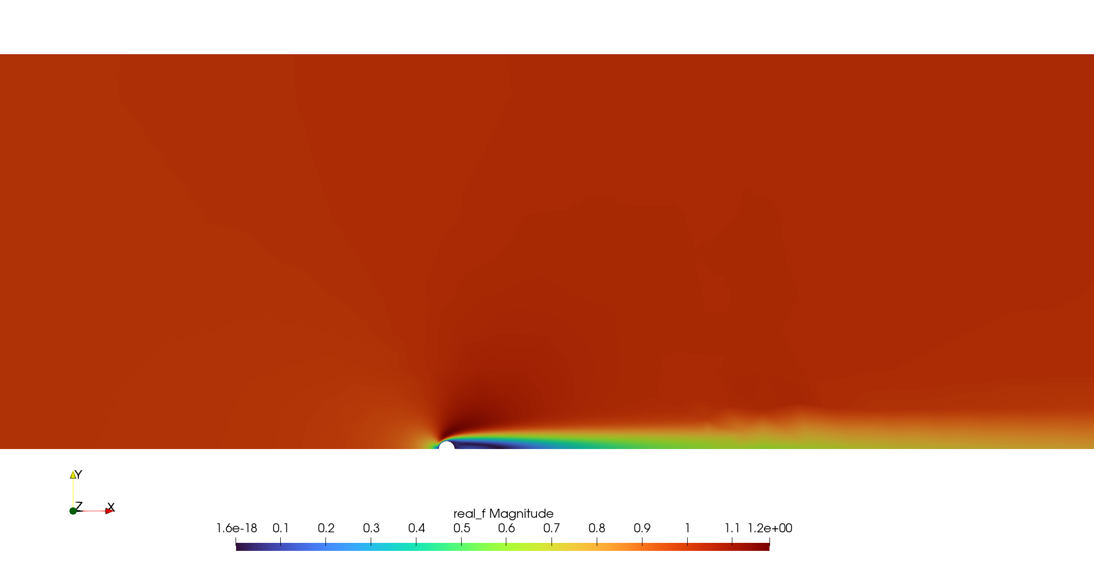Figure 3. Magnitude of the flow-field.