Tutorial 3: Resolvent Analysis

Goal of the Tutorial

The goal of this tutorial is to provide a step-by-step guide on performing resolvent analysis in FELiCS. By the end of this tutorial, you will be able to:

• Write a mesh file on GMSH using a python script.

• Import the mean flow data and create a mean flow file for FELiCS.

• Perform resolvent analysis for different frequencies.

• Plot the gains and mode shapes in Python.

The resolvent analysis provides insights into:

• (Dominant) amplification mechanisms of harmonic perturbations in the flow, quantified by a frequency dependent gain function

• In which flow region these amplification mechanisms are most efficiently triggered (optimal forcings mode)

• What it the response to a optimal forcing (optimal response mode)

The resolvent analysis will:

1. Identify frequencies and spatial regions where the flow is most sensitive to forcing.

2. Quantify the gain between input disturbances and flow response for each frequency.

Case Definition

In this tutorial, we will perform incompressible resolvent analysis about the 2D mean flow in a constricted pipe (stenosis). For the geometry details, see Villié et al. 2025. The inlet has a steady inflow boundary condition with a Reynolds number of 8000 based on the diameter and bulk speed in the contraction. Since the mean flow is axisymmetric, the 3D solution is solved for a given azimuthal wavenumber.

Mesh generation

We generate the 2D mesh on GMSH. To do so, we write a .geo file readable by GMSH using the python script geoMesh.py.

Feel free to play with the CellsFineness factor to see the influence of finer meshes.

Open the .geo file with GMSH an click on ‘Mesh -> 2D’. You should obtain this mesh: 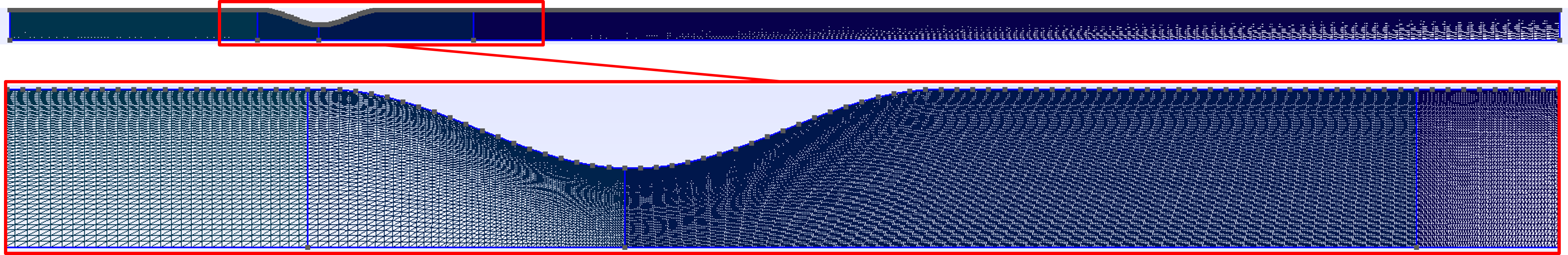Figure 1. Stenosis mesh Export the mesh in File -> Export in a .msh format with Version 2 ASCII. Place this FELiCS_mesh.msh file in your case folder.

Base Flow

This tutorial case folder is located in felics/tutorials/resolvent_tutorial. Our base flow is obtained by time-azimuthal-averaging the snapshots of a 3D LES. Alternatively this could be a RANS solution, experimental data, or any other relevant flow field. Run the python script meanFlow.py to load the mean flow data and write a .fel file. Change the fold_path to your data folder and run the script. This script also allows to define response and forcing domains, a sponge function and an eddy viscosity field. In our case, the response and forcing domains are the same, but we could restrict it to different regions. The sponge function is used to dampen the fluctuations near the inlet/outlet.

Place the meanFlow.fel file in your case folder.

Resolvent parameters

Boundary conditions

Here, we set the axisymmetric boundary conditions in the boundaries.json file. First check in your readable .msh file the boundary ids. For instance in this file:

$MeshFormat
$PhysicalNames
5
1 2 "centerline"
1 3 "inlet"
1 4 "outlet"
1 5 "walls"

the IDs of “centerline”, “inlet”, “outlet”, “walls” are respectively 2,3,4,5.

Define the boundaries in the file boundaries.json using the corresponding IDs. The file structure is detailed in Setting files. In our case, we set:

Boundary	\(u'_x\)	\(u'_r\)	\(u'_\theta\)	\(p'\)
Symmetry	Neumann	Dirichlet	Dirichlet	Dirichlet
Inlet	Dirichlet	Dirichlet	Dirichlet	Dirichlet
Outlet	Dirichlet	Dirichlet	Dirichlet	Dirichlet
Wall	Dirichlet	Dirichlet	Dirichlet	Neumann

Settings

The setting file resolvent_settings.json contains all the analysis information. The explanation of each field is provided in Setting files.

Here are some key settings for our resolvent analysis:

• The coordinates system is set to Cylindrical:

{"CoordinateSystem": "Cylindrical",}

Note

The velocity components are thus refered to as ux, ur, ut instead of ux, uy, uz. ‘’’

• We choose to study axisymmetric perturbations by setting the azimuthal wavenumber to 0:

    "m":0.0,

• Since we non-dimensionalized the state variables, equations and the mesh/cmoputational domain, we set the molecular viscosity \(\nu\) to be the inverse of the Reynolds number:

"MolVisc":0.000125,

You can increase this field in order to add a uniform eddy viscosity field.Ensure consistency in the normalization approach throughout the analysis.

• We want to solve the Momentum and Mass equations only and set the other equations in ”SetofEquations” to "None"

• If we included a turbulent viscosity field in the meanFlow.py file, we should set:

    {"TurbulenceModel":"File"}

• The frequencies for which we compute the resolvent modes are provided in the field:

    {"Omegas":[0.062, 0.10, 0.17, 0.29, 0.48, 0.81, 1.35, 2.26, 3.1, 4.36, 6.28]}

• We can vary the number of resolvent modes that we want to compute with the field:

    {"nSolut": 2}

Note

The following fields CalculateAdjoint and EigenValueGuess are not relevent for the resolvent analysis.

Running the analysis

Your case folder should look like:

.
├ FELiCS_mesh.msh
├ meanFlow.fel
├ resolvent_settings.json
├ boundaries.json
└ mixture.json

Run the analysis with the command:

FELiCS -f resolvent_settings.json

With the provided mesh, it should take about two minute to compute the two resolvent modes for each frequency (~25 minutes).

Postprocessing

After the computation, the output_dir/ has been created. You will find there the following files:

.
└── output_dir
    ├ gains.csv
    ├ MeanFlow.h5
    ├ MeanFlow.xmf
    ├ mesh.h5
    ├ Mode_Resolvent_Forcing_Omega_3.1_GainNb_0.xmf
    ├ Mode_Resolvent_Forcing_Omega_3.1_GainNb_0.h5
    ├ Mode_Resolvent_Response_Omega_3.1_GainNb_0.xmf
    ├ Mode_Resolvent_Response_Omega_3.1_GainNb_0.h5
    └ ...

We postprocess the outputed files using the python script PlotMode.py.

Modify the defined path to your folder and run the script.

The resolvent gains are plotted against the Strouhal number \(St = \omega/2\pi\) in Figure 2.

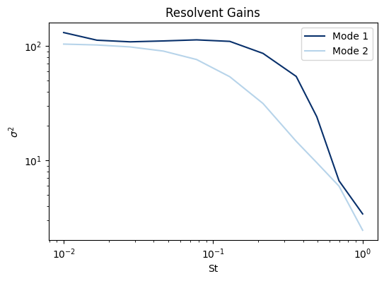
Figure 2. Resolvent gains Note that in this case, only the leading and first subleading resolvent modes were computed.

The script also include functions to read the mesh, load and plot the mode in matplotlib. The forcing and response mode shapes for \(p', u_x', u_r'\) at \(\omega = 3.1\) are plotted in Figure3 and Figure4, respectively:

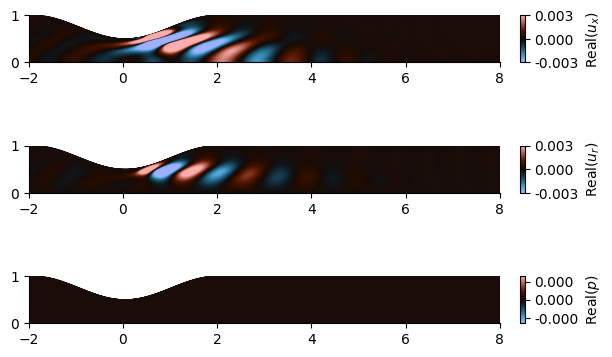
Figure 3. Forcing mode shape

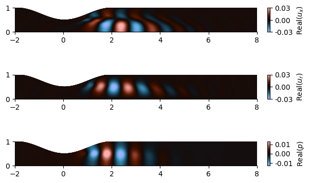
Figure 4. Response mode shape

The \(u_\theta\) fluctuation is 0 in this case because we study axisymmetric perturbations (\(m=0\)).

Warning

The gains provided by FELiCS are \(\sigma^2\). The forcing modes have a unitary norm on the defined forcing domain, but the response modes have the norm \(\sigma\) on the defined response domain.