How to load modes from a FELiCS run and compute structural sensitivity#
Before you start, you should install all necessary FELiCS packages, and install FELiCS as a package itself. The installation guide explains those steps in detail.
After installing FELiCS you can start writing your first FELiCS script.
This tutorial explains how to load previously computed resolvent or eigenmodes from disk using the FELiCS I/O module. The results were saved in the /Input directory. For more information about the initial computation of modal results, see the how-to guide #3.
1. Imports and configuration
We begin by importing the necessary FELiCS modules and reading the simulation configuration.
from 	FELiCS.Parameters.Config	        import 	Config
from 	FELiCS.Misc.logging			        import  Logger
from    FELiCS.IO.Reader                    import  Reader
from    FELiCS.Fields.Field                 import  Field
from    FELiCS.SpaceDisc.FEMSpaces          import  FEMSpaces
from    FELiCS.Fields.ModeCollection        import  ModeCollection
import  ufl
from    FELiCS.Misc.tensorUtils             import Tensor, i_dot, i_conj


🔧 Set up logging and read configuration


```python
logger = Logger(True, False, "felics")
logger = Logger.get_logger("felics")

param = Config()
param.import_from_file("Input/config.json")
Debug    | logging.py             | _setup_logger              (line 245 ) : Logger initialized successfully
Debug    | Config.py              | __init__                   (line 68  ) : Initializing config class with defaults.
Info     | Config.py              | import_from_file           (line 245 ) : Loading configuration from Input/config.json
Warning  | Config.py              | import_from_file           (line 264 ) : Field "MolViscPerturbModel" missing from file, setting default: {'type': 'Constant', 'Constants': {'Viscosity': 1.0}}
Warning  | Config.py              | import_from_file           (line 264 ) : Field "PrandtlNumber" missing from file, setting default: 0.72
Warning  | Config.py              | import_from_file           (line 264 ) : Field "ForcingNorm" missing from file, setting default: TKE
Warning  | Config.py              | import_from_file           (line 264 ) : Field "ResponseNorm" missing from file, setting default: TKE
Debug    | Config.py              | import_from_file           (line 273 ) : Checking mandatory files
Info     | logging.py             | change_log_location        (line 364 ) : Log files moved to: Input/OutModal/log
Debug    | Config.py              | import_from_file           (line 292 ) : Creating Mixture class
Info     | MixtureClass.py        | __init__                   (line 101 ) : No mixture file Mixture.json, using defaults.
Debug    | Config.py              | read_domain_data           (line 503 ) : Reading domain data from 'Input/CylinderWakeMesh.msh'
Info     | FELiCSMesh.py          | __init__                   (line 124 ) : Opening mesh file: Input/CylinderWakeMesh.msh
Info     | FELiCSMesh.py          | __init__                   (line 132 ) : Mesh contains 3613 nodes and 7224 elements
Debug    | FELiCSMesh.py          | __init__                   (line 194 ) : The transverse/azimuthal wavenumber is m=0.0 and the geometric dimension is gdim=2.
Debug    | FELiCSMesh.py          | __init__                   (line 199 ) : Setting true dimension to self.dim=2 (geometric dimension)
Info     | Config.py              | import_from_file           (line 314 ) : Configuration loaded successfully
This creates:
a global FELiCS logger
a
paramobject that contains all case parameters (mesh path, polynomial order, Reynolds number, etc.), loaded fromconfig.json.
2. Initialization of core FELiCS objects
In this section we reconstruct the essential FELiCS objects exactly as they were used during the mode computation. This ensures consistency of function spaces and mesh mappings.
mesh = param.get_mesh()
FELiCS loads the mesh using the path and options specified in config.json.
FEMSpaces = FEMSpaces(param, mesh)
Info     | FEMSpaces.py           | __init__                   (line 174 ) : Defining FEM-spaces.
Debug    | FELiCSMesh.py          | __init__                   (line 469 ) : Initializing refined P1 export mesh.
Debug    | FELiCSMesh.py          | __init__                   (line 194 ) : The transverse/azimuthal wavenumber is m=0 and the geometric dimension is gdim=2.
Debug    | FELiCSMesh.py          | __init__                   (line 199 ) : Setting true dimension to self.dim=2 (geometric dimension)
Debug    | FEMSpaces.py           | __init__                   (line 235 ) : Adding FEM space of order 2 for u
Debug    | FEMSpaces.py           | __init__                   (line 235 ) : Adding FEM space of order 2 for p
Debug    | FEMSpaces.py           | __init__                   (line 253 ) : Mixed finite element list: [blocked element (Basix element (P, triangle, 2, gll_warped, unset, False, float64, []), (2,)), Basix element (P, triangle, 2, gll_warped, unset, False, float64, [])]
This initializes the mixed finite-element space used for the velocity and pressure variables. These spaces must match the ones used when the modes were originally computed.
📥 Initialize the Reader and Writer
reader = Reader(
    sourceDir="Input",
    needInterpolation=False,
)
The Reader searches the Input/ directory for mode files written by a previous FELiCS run.
3. Loading modes from disk
FELiCS stores modes in an organized modeCollection structure. To load all modes at once, we create an empty ModeCollection and call its importData method.
ModeCollection manages groups of modes, facilitates filtering, and provides utility functions (descriptions, sorting, exporting, etc.).
FELiCS will automatically:
scan the folder
detect available modes (direct and/or adjoint)
reconstruct each mode as a Mode object
rebuild all subfields in the correct function spaces
attach metadata (type, eigenvalue, iteration number, etc.)
importSolution = ModeCollection(
    FEMSpaces.VMixed,
    mesh
)
importSolution.import_data(
    reader,
    "Input",
)
Info     | ModeCollection.py      | import_data                (line 932 ) : 2 modes to import into mode collection.
Info     | ModeCollection.py      | import_data                (line 934 ) : Importing mode 1/2 from file "Mode_Modal_Direct_Omega_0.727+0.001j.h5".
Debug    | Reader.py              | _update_calc_mesh          (line 459 ) : New calculation mesh / FEM space type, updating cache.
Debug    | Reader.py              | clear_cached_properties    (line 561 ) : No cached properties to clear.
Debug    | Reader.py              | import_mesh_coords         (line 267 ) : Associating import mesh to Reader instance.
Debug    | Reader.py              | import_mesh_coords         (line 272 ) : Getting the 2D import mesh coordinates (['x', 'y']).
Debug    | Reader.py              | import_mesh_coords         (line 335 ) : Executing Option 3: No interpolation needed: load from FELiCS exported mesh file.
Debug    | Reader.py              | import_mesh_coords         (line 346 ) : self._felicsMeshFilePath is None, therefore using Input/mesh.h5
Debug    | Reader.py              | _update_data_source        (line 406 ) : Reader: switched source to ('/Users/marina/Documents/repositories/FELiCS/how_tos/04_LoadingModesAndStructuralSensitivity/Input/Mode_Modal_Direct_Omega_0.727+0.001j.h5', None), cleared per-file caches.
Debug    | Reader.py              | import_in_field            (line 1013) : Cache empty, loading and interpolating/mapping all available data: ['p_imag', 'p_real', 'ux_imag', 'ux_real', 'uy_imag', 'uy_real']
Debug    | Reader.py              | import_in_field            (line 1053) : Getting ['ux', 'uy', 'p'] from cached data.
Info     | ModeCollection.py      | import_data                (line 967 ) : Imported mode 1/2 from "Mode_Modal_Direct_Omega_0.727+0.001j.h5".
Info     | ModeCollection.py      | import_data                (line 934 ) : Importing mode 2/2 from file "Mode_Modal_Adjoint_Omega_0.727-0.001j.h5".
Debug    | Reader.py              | _update_data_source        (line 406 ) : Reader: switched source to ('/Users/marina/Documents/repositories/FELiCS/how_tos/04_LoadingModesAndStructuralSensitivity/Input/Mode_Modal_Adjoint_Omega_0.727-0.001j.h5', None), cleared per-file caches.
Debug    | Reader.py              | import_in_field            (line 1013) : Cache empty, loading and interpolating/mapping all available data: ['p_imag', 'p_real', 'ux_imag', 'ux_real', 'uy_imag', 'uy_real']
Debug    | Reader.py              | import_in_field            (line 1053) : Getting ['ux', 'uy', 'p'] from cached data.
Info     | ModeCollection.py      | import_data                (line 967 ) : Imported mode 2/2 from "Mode_Modal_Adjoint_Omega_0.727-0.001j.h5".
🔍 Inspect loaded modes This prints a summary of the imported modes: mode numbers, types, eigenvalues, …
importSolution.describe()
Info     | ModeCollection.py      | describe                   (line 105 ) : ModeCollection for AnalysisType.MODAL analysis.
Info     | ModeCollection.py      | describe                   (line 106 ) : Contains 2 modes. Contents:
Info     | ModeCollection.py      | describe                   (line 110 ) :   Mode 0:
Info     | Mode.py                | describe                   (line 471 ) :   Mode Type:     DIRECT
Warning  | Mode.py                | guess                      (line 410 ) : For this mode object no guess was defined. Returning "-9999."...
Info     | Mode.py                | describe                   (line 473 ) :   Guess:         -9999.0
Info     | Mode.py                | describe                   (line 474 ) :   Eigenvalue:    (0.7273431802447553+0.0012707477677050048j)
Info     | Mode.py                | describe                   (line 481 ) :   Wave Number:   0
Info     | ModeCollection.py      | describe                   (line 110 ) :   Mode 1:
Info     | Mode.py                | describe                   (line 471 ) :   Mode Type:     ADJOINT
Warning  | Mode.py                | guess                      (line 410 ) : For this mode object no guess was defined. Returning "-9999."...
Info     | Mode.py                | describe                   (line 473 ) :   Guess:         -9999.0
Info     | Mode.py                | describe                   (line 474 ) :   Eigenvalue:    (0.7273431802447646-0.001270747767560071j)
Info     | Mode.py                | describe                   (line 481 ) :   Wave Number:   0
4. Extracting specific modes and fields Most analyses involve separating direct and adjoint modes, then selecting individual components of the state vector.
🎯 Separate direct and adjoint modes
directMode  = [m for m in importSolution.modeList if m.modeType.name == "DIRECT"][0]
adjointMode = [m for m in importSolution.modeList if m.modeType.name == "ADJOINT"][0]
You can always check:
print(directMode.modeType.name)
DIRECT
🔬 Accessing subfields
FELiCS organizes the mixed state vector hierarchically:
Mode
└── Velocity field
└── Streamwise component (u)
└── Transverse component (v)
└── Pressure
└── … (other fields depending on the model)
To extract the streamwise velocity:
uxFieldDirect  = directMode.get_list_of_sub_fields()[0].get_list_of_sub_fields()[0]
uxFieldAdjoint = adjointMode.get_list_of_sub_fields()[0].get_list_of_sub_fields()[0]
Here:
getListOfSubFields()[0]→ the velocity vector...getListOfSubFields()[0]→ first component, i.e. streamwise velocity
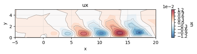
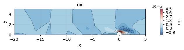
5. Plotting the modes
Each scalar field knows how to plot itself using Matplotlib and the triangulation utilities integrated in FELiCS.
uxFieldDirect.plot(xlim=(-5, 20), ylim=(0, 5))
uxFieldAdjoint.plot(xlim=(-20, 5), ylim=(0, 5))
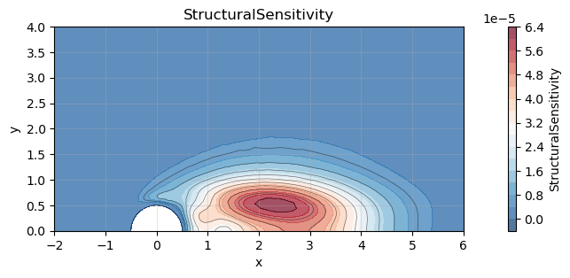
6. 🌋 Structural Sensitivity in FELiCS
In global stability analysis, the structural sensitivity — often called the wavemaker — identifies the regions in the flow where small changes in the operator have the strongest impact on the eigenvalue. This is precisely the region where an instability is born.
This concept was introduced in the seminal paper: Giannetti & Luchini (2007), “Structural sensitivity of the first instability of the cylinder wake” Journal of Fluid Mechanics, 581: 167–197. doi: 10.1017/S0022112007005654
Their analysis showed that, at the Hopf bifurcation of the cylinder wake, the wavemaker is a compact bubble located just downstream of the cylinder, at the intersection between:
regions where the direct mode is energetic (perturbation amplification), and
regions where the adjoint mode is energetic (flow receptivity). Understanding this overlap region is essential for model reduction, flow control, and sensitivity-based design.
📐 (Abbreviated) Mathematical definition Given a direct velocity mode \(u_d(x)\) and the corresponding adjoint mode \(u_a(x)\), the structural sensitivity tensor is
Its Frobenius norm is a scalar field that gives the maximum possible structural sensitivity in each point:
🛠️ How to evaluate tensor expressions in FELiCS (essentials)
evaluateUflTensorExpression is a compact but powerful FELiCS routine that evaluates any tensor-based UFL expression and stores the result in a Field. It is the recommended way to compute derived quantities (e.g. structural sensitivity, vorticity, energy norms) because it:
✔ Uses the FELiCS tensor framework: The expression is interpreted using
Tensor,iDot,iConj, and the coordinate-system JacobianJ_hat, ensuring that all operators follow the correct physics, including non-Cartesian coordinate systems and spectral directions. (A pure-ufl version of this function exist withevaluateUflExpression)✔ Automatically assembles a consistent weak form: The method builds the appropriate “mass-like” variational form for the field’s function space, assembles it once, and stores the corresponding LU solver for reuse.
✔ Efficiently evaluates and inserts the result: The input expression is assembled into a vector, solved with the precomputed solver, and the field’s coefficient array is updated.
✔ Ideal for post-processing: You can turn complex mathematical expressions directly into FEM fields with one line, without manually writing projection operators or variational problems.
🧠 Structural sensitivity in FELiCS FELiCS uses a tensor-aware framework for field representation. This allows us to compute expressions like structural sensitivity in a coordinate-system consistent way.
The computational steps are:
🔍 Extract the direct and adjoint velocity fluctuation fields.
🧮 Choose a scalar FE space \(V\) to store the sensitivity.
✏️ Build the appropriate UFL tensor expression
⚙️ Assemble the expression using
evaluateUflTensorExpression.🎨 Plot the resulting scalar field.
🧩 FELiCS implementation
# --- Extract direct and adjoint velocity fields -----------------------
uFieldDirect  = directMode.get_list_of_sub_fields()[0]   # velocity fluctuation
uFieldAdjoint = adjointMode.get_list_of_sub_fields()[0]

# --- Test space where the scalar sensitivity will live ---------------
V_scalar = FEMSpaces.P2
v        = ufl.TestFunction(V_scalar)

# --- Create empty field to store structural sensitivity --------------
sS       = Field(V_scalar, mesh)
sS.name  = "StructuralSensitivity"

# --- Build the UFL tensor expression ---------------------------------
J_hat  = sS.mesh.coordinate_system.J_hat

v_tens = Tensor(
    v,
    CoordSys=sS.mesh.coordinate_system,
    m=sS.m,
    mayHaveSpectralDimension=sS.hasSpectralDimension,
)

exprSS = (
    i_dot(uFieldDirect.get_tensor(),  i_conj(uFieldDirect.get_tensor()))**0.5 *
    i_dot(uFieldAdjoint.get_tensor(), i_conj(uFieldAdjoint.get_tensor()))**0.5 *
    i_conj(v_tens)
).ufl_tens * J_hat * ufl.dx

# --- Evaluate expression and build the finite-element field -----------
sS.evaluate_ufl_tensor_expression(exprSS)
🎨 Plotting the result
sS.plot(xlim=(-2, 6), ylim=(0, 4))