How to calculate the spatial gradient of a scalar field in cylindrical coordiantes

Step 1: Create FELiCSMesh, FELiCSSpace and Field

Cylindrical coordinates:

FELiCS is able to handle cartesian and cylindrical coordinates. The cylindrical coordinates in FELiCS are defined with (x, r, theta) where x is analogous to the x in cartesian coordinates, r is the radial component (distance from x-axis) and theta is the azimuthal/angular coordinate which is the angle around the x-axis. with this coordinate choice our square mesh is basically “rolled” into a cylinder.

TODO put equation of gradient with derivative w.r.t. spectral dimension (if any doubt, see https://en.wikipedia.org/wiki/Del_in_cylindrical_and_spherical_coordinates)

from FELiCS.SpaceDisc.FELiCSMesh import FELiCSMesh
from FELiCS.IO.Reader            import Reader
from FELiCS.SpaceDisc.FEMSpaces  import createFunctionSpace
from FELiCS.Fields.Field         import Field

meshFileName = "./square_mesh.msh"
coordinateSystemName = "Cylindrical"
m = 3

# Create a FELiCS mesh from the gmsh file
mesh = FELiCSMesh(coordinateSystemName, meshFileName)

space = createFunctionSpace(mesh, degree=2, dim=1)

phi = Field(space, mesh, name="function_sine_cos") 
phi.importData(Reader(), "input.h5")

Info     | FELiCSMesh.py          | __init__                   (line 75  ) : Opening mesh file: ./square_mesh.msh
Info     | FELiCSMesh.py          | __init__                   (line 83  ) : Mesh contains 513 nodes and 1024 elements





(<FELiCS.Fields.Field.Field at 0x7fcd431458b0>, [])

Step 2: Calculate the gradient

We now want to calculate the gradient of our scalar quantity using the getGradient() method of our Field class. This method returns a Field

gradPhi = phi.getGradientField()

Step 3: Postprocessing

Visualization of the gradients with

gradPhiList = gradPhi.getListOfSubFields()
phi_x = gradPhiList[0]
phi_r = gradPhiList[1]
phi_x.plot()
phi_r.plot()

Cylindrical coordinates with spectral dimension

Here, to the two spatial dimensions (x and r) a third spectral dimension in theta-direction is added. With the spectral dimension the scalar field becomes

\[\phi \cdot e^{im\theta}\]

where m is the wave number. With the wave number we represent a periodicity of the flow in theta-direction, while still only calculating a 2D flowfield.

Step 1: Create FELiCSMesh, FELiCSSpace and Field

from FELiCS.SpaceDisc.FELiCSMesh import FELiCSMesh
from FELiCS.SpaceDisc.FEMSpaces  import createFunctionSpace
from FELiCS.Fields.Field         import Field
from FELiCS.IO.Reader            import Reader

meshFileName = "./square_mesh.msh"
coordinateSystemName = "Cylindrical"
m = 2

# create a FELiCS mesh from the gmsh file
# by setting m to an integer number that is not zero, the spectral direction is added to the coordinate system
mesh = FELiCSMesh(coordinateSystemName, meshFileName, m=m) 

# create a scalar space
scalarSpace = createFunctionSpace(mesh, degree=2, dim=1)

# create a Field object and import the data from the h5 file
# by setting m to an integer number that is not zero, the spectral direction is added to the field
phi = Field(scalarSpace, mesh=mesh, name = "function_sine_cos", m = m) 
phi.importData(Reader(),"input.h5")

Info     | FELiCSMesh.py          | __init__                   (line 75  ) : Opening mesh file: ./square_mesh.msh
Info     | FELiCSMesh.py          | __init__                   (line 83  ) : Mesh contains 513 nodes and 1024 elements





(<FELiCS.Fields.Field.Field at 0x7fcd3a5ca750>, [])

Step 2: Calculate the gradient

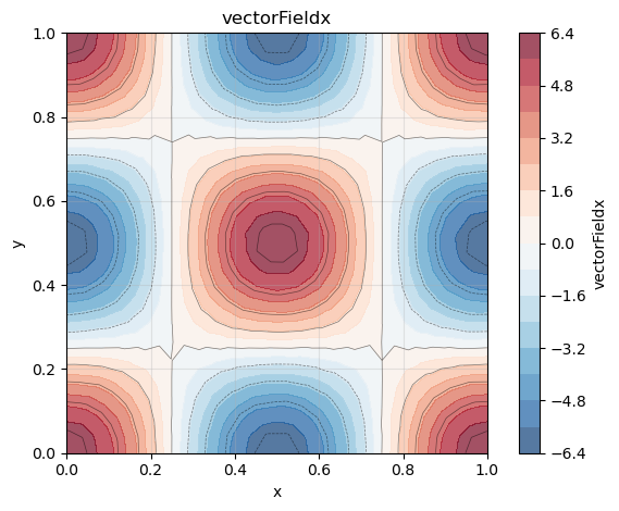
With the spectral dimension, the gradient is now 3-dimensional:

\[\nabla \phi = \left(...\right)\]

and it is defined as:

\[\begin{split}\nabla \phi = \begin{pmatrix} ... \\ ... \\ ... \end{pmatrix}\ .\end{split}\]

gradPhi = phi.getGradientField() # this is a vector field

# get scalar fields from gradient:
gradList = gradPhi.getListOfSubFields()
phi_x    = gradList[0]
phi_r    = gradList[1]
phi_t    = gradList[2]

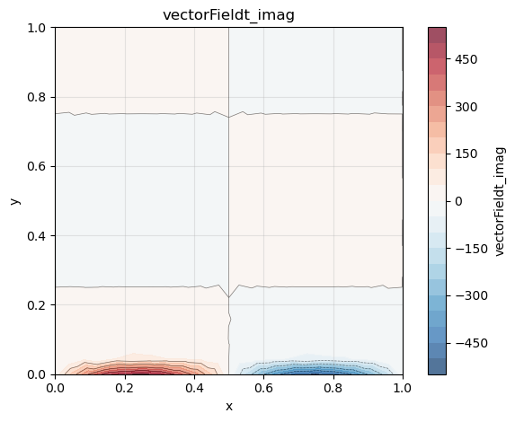
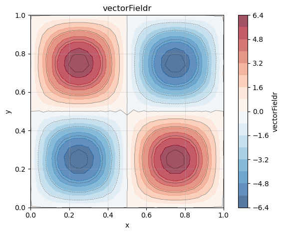
Step 3: Postprocessing

Exporting as h5 file and visualization of the gradients by using the FELiCS plotting function:

from FELiCS.IO.Writer import Writer
gradPhi.exportToH5(Writer())

phi_x.plot()
phi_r.plot()
phi_t.plot(imaginaryPart=True)