How to calculate the vorticity of a 2D field#
Step 1: Create FELiCSMesh, FELiCSSpace and Field
We consider the domain \(\Omega = (0,1) \times (0,1)\), and discretize with triangular elements. The 2D velocity field is a \(P2\) finite element vector field and the magnitude of the vorticity has been stored in a \(P2\) finite element scalar field.
from FELiCS.SpaceDisc.FELiCSMesh import FELiCSMesh
from FELiCS.SpaceDisc.FEMSpaces  import create_function_space
from FELiCS.Fields.Field         import Field
from FELiCS.IO.Reader            import Reader

meshFileName = "./square_mesh.msh"
coordinateSystemName = "Cartesian"

# Create a FELiCS mesh from the gmsh file
mesh = FELiCSMesh(coordinateSystemName, meshFileName)

scalarSpace = create_function_space(mesh, degree=2, dim=1)
vectorSpace = create_function_space(mesh, degree=2, dim=2)

phiVec = Field(vectorSpace, mesh=mesh, name="function_2d")
phiVec.import_data(Reader(), "input")
Info     | FELiCSMesh.py          | __init__                   (line 124 ) : Opening mesh file: ./square_mesh.msh
Info     | FELiCSMesh.py          | __init__                   (line 132 ) : Mesh contains 513 nodes and 1024 elements
Info     | Reader.py              | _interpolate_to_calc_mesh  (line 706 ) : Linear interpolation took 0.6 seconds. (Mesh size: (1969, 2))


(<FELiCS.Fields.Field.Field at 0x1645e3770>, [])
Step 2: Computing the vorticity and comparison with the analytical results.
For a 2D velocity field given by \(\vec{\textbf{u}} = (u, v)\), the vorticity \(\omega\) is defined as
where \(\hat{x}, \hat{y}, \hat{z}\), represent the unit vectors along the Cartesian coordinate axes in 3D space. However, for a 3D velocity field given by \(\vec{\textbf{u}} = (u, v, w)\), the vorticity \(\omega\) is defined as
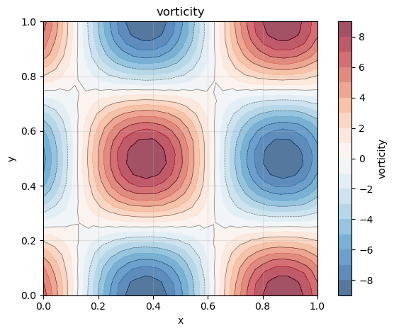
vorticity = phiVec.get_vorticity_field()
Step3. Postprocessing via plotting contour plots
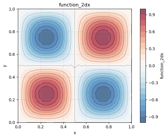
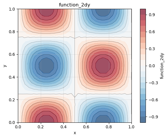
We plot two 2D color plots of the velocity and vorticity magnitudes respectively.
[phi_x, phi_y] = phiVec.get_list_of_sub_fields()

phi_x.plot()
phi_y.plot()
vorticity.plot()